Lab 11: Operating an Unmanned Aerial System

Introduction

An unmanned aerial system (UAS) is a term that encompasses all components required in the operation of a drone including the drone itself, the pilot, and the support equipment. This lab was a basic introduction to operating a drone and some of the ethics of their use. 

Drone Basics

The drone that was flown in this lab consisted of four blades, a center console, and the camera (figure 1).

Figure 1. Drone flown on May 8, 2018.

The camera that is placed on the bottom of the drone can vary from a high resolution camera to a red edge device which is used to monitor vegetation health. The drone in figure 1 is sitting on four legs that are part of the landing gear. These will retract once the drone is in flight. 

Before the drown is flown, two calibrations must be made: compass calibration and lens calibration. The compass calibration orients the GPS unit on the drone so accurate location points are taken. The lens calibration ensures accurate imagery is recorded. 

Once these two processes are complete other settings can be adjusted such as side and end lap. Side lap is the intersection between adjacent images in different flight lines and end lap is the intersection between images in the same flight line. This can be thought of as side-to-side and front-to-back overlay. The mission must also be loaded. This is the area that one wants to be imaged by the drone. This information will be loaded into the drone and the drone will then fly itself over the intended area. 

In more advanced missions, there will be a master controller who controls the flight of the drone and other aspects and the slave controller that controls the camera. 

A final point worth mentioning is ethics. There is a lot of controversy about whether drone owners should have to register their device. Current technology allows drones to fly into spaces otherwise inaccessible and can obtain imagery that some maintain is an invasion of privacy. Many professional drone fliers with licenses choose to follow the code of ethics but many hobby drone fliers choose not to. 

Drone Operation

The following is a video of the drone taking off.

During the mission flight of the drone, the user simply has to watch to ensure that the drone does not deviate from its intended course and monitor its progress. This can be done via the controller screen (figure 2).

Figure 2. Controller screen while the drone was in use.

Once the mission was completed the drone flew back to its original takeoff point and landed.

The actual flying of the drone was relatively simple. Once the mission was completed each student was allowed to fly the drone manually (figure 3). 

Figure 3. Lindsey Kurtz flying the drone.

The controls allowed the user to bring the drone higher or lower in elevation or in any of the cardinal directions. 

Conclusion

Overall this lab was a very simple introduction to operating a drone. There are many more components that make up a UAS system. As UAS technology becomes even better, UAS will be implemented in more and more areas such as precision agriculture and security. This exercise was a great introduction into the operation of a UAS system.

Lab 10: Distance Azimuth Survey

Introduction

Sometimes technology can fail in the field and another method is needed to complete the work. This lab introduced the distance azimuth survey, a basic survey technique that can come in handy if such a circumstance arises. This sampling technique is related to others such as the point-quarter method or mapping out linear features on the landscape. In this lab groups of three to four students went out to Putnam drive on the University of Wisconsin-Eau Claire campus and completed a tree survey to practice the distance azimuth survey technique. The data was then inputted to ArcMap and transformed into a feature class that could be further analyzed.

Study Area

The study area was located on Putnam Drive behind the University of Wisconsin-Eau Claire (figure 1).

Figure 1. Putnam Drive in Eau Claire, WI where the tree survey was completed.

This area is populated with both dry and wet soil trees. The area directly adjacent to the parking lot behind Davies Center on campus is a small swamp with a small stream flowing along its border. Across the swamp is a gravel trail accessible to cars and bikers. Beyond this trail is the steep incline that leads to the former flood plain of the Chippewa River called the Wissota Terrace, or better known as upper campus. The swamp area has wet soil species such as river birch and ash trees. The steep incline leading to upper campus has a drier soil due to water running to lower elevation areas. This section of Putnam trail is home to dry soil species such as red oak and basswood trees. The trees selected for this tree survey were located in both areas. Trees selected for the survey were chosen based on distance from the reference point (had to be feasible to measure the distance from reference point) and the tree type (several tree types were desired for the survey).

Methods

The attributes collected for each point were chosen before sampling to ensure usable data was collected. In this survey, 17 trees were sampled. The location column in the data was recorded for the reference point and thus was the same for the first 12 trees and again for the remaining 5 due to the nature of the distance azimuth survey. In addition, the distance from the reference point, azimuth (degree angle from north), tree type, and circumference were all recorded for each tree. The azimuth and distance will be described shortly in the survey process. Tree type and circumference were chosen as tree characteristics that could later be analyzed spatially for any patterns on the maps in relation to topography and soil type

The process for collecting each tree sample was as follows. First, a reference point was established. The coordinates for this point were obtained using Bad Elf GPS and an iPhone. Bad Elf was used to collect the second reference point as well (figure 2).

Figure 2. Bad Elf GPS device used with an iPhone to obtain reference point coordinates.

Next, a tree was chosen based on location and tree type. The tree was identified based on its bark and leaves. Once the tree was chosen, a tape measure determined the circumference of the tree in centimeters. Then, the tape measure was used to determine the tree’s distance from the reference point (figure 3).

Figure 3. Tape measure used to determine the distance of each tree from the reference point. The reference point is located where the two individuals are standing in the background.

For some tree distances, a laser was used but it was found to be more inaccurate than the tape measure so its use was discontinued. Finally, the azimuth was determined using a field compass (figure 4).

Figure 4. Azimuth compass used to determine the azimuth of each tree sample.

By looking through the azimuth compass, the degree measure from north, or 0 °, can be accurately obtained as demonstrated in figure 5.

Figure 5. Azimuth compass used by Luke Burds to obtain an azimuth reading.

Figure 6 shows the complete table of all measurements taken in the field. The left page describes what each symbol represents for the tree types in the table on the right-hand page.

Figure 6. Field notebook including all data obtained for each tree sample.

With this information and the distance from the reference point, the x, y coordinates can be obtained in ArcMap. 

The final step was to import the data into an excel file and then to ArcMap and run two tools: Bearing Distance to Line tool and Feature Vertices to Points tool. Both of these tools are located in the ‘data management tool box’ and under the ‘feature’ subset. The bearing distance to line command creates a new feature class containing geodetic line features constructed based on x, y, azimuth, and distance values. In other words, lines from the reference point are plotted based on the x, y coordinates of the reference point and the azimuth and distance of each tree surveyed. This tool also allows the user to import other attribute data field information such as the tree type.

Next, the Feature Vertices to Points tool created a feature class containing points generated from the specified locations at the ends of the lines that were created with the previous tool. This then creates a point feature class that contains all the pertinent attribute data that can be used for querying in the future. 

Results/Discussion

Figure 7. Map of lines from the reference point to each tree location. There were two separate data groups.

Figure 7 shows the line feature class that was created using the bearing distance to line tool. Each line originates from the reference point and ends at the tree location. This feature class lines up with survey data taken.

Figure 8. Map of tree locations in Putnam Drive. These locations were derived from the locations denoted at the ends of the lines in the map in figure 7.

Figure 8 shows the final points depicting tree locations. The points are fairly accurate based on the basemap imagery. Some of the tree sampled down in the swamp area appear to be on the path, but this discrepancy could be due to the change in elevation not included in the basemap.  In particular, the points are very accurate location-wise from the reference point. This accuracy and overall accuracy in the real-world indicate that the measurements were accurate as were the GPS coordinates.

Figure 9. Tree types denoted by color. No apparent trends are seen in the data.

Figure 9 shows the tree types of the 17 trees sampled in the survey. The sample size is quite small, so no trends such as wet vs. dry soil tree types appear in the data.  However, there was one river birch in the right-hand sample and two black walnut in the left-hand sample. Both these trees did occur at a lower frequency than the other types of trees based on a visual analysis of the area.

Conclusion

Overall this lab was effective in providing experience in performing a distance azimuth survey. This technique is beneficial because it can be used in the field when other forms of technology are unavailable and can also be very accurate as the results showed. A survey would take more time if the objects were a farther distance away than 20 meters. This used to be the standard technique used in the field to collect data. Today, survey-grade GPS units have replaced this method with accurate locations down to the centimeter in certain cases. GPS units today can also do post-processing in addition to gathering the initial data. While easier methods for obtaining field data are available, the distance-azimuth method is still a valuable tool in obtaining data if technology fails (which it can and will) in the field.

Sources

“Bearing Distance to Line.” (2018). Accessed April 24, 2018. http://pro.arcgis.com/en/pro-app/tool-reference/data-management/bearing-distance-to-line.htm

“Feature Vertices to Points.” (2018). Accessed April 24, 2018. http://pro.arcgis.com/en/pro-app/tool-reference/data-management/feature-vertices-to-points.htm

Lab 9: Arc Collector Research Project

Introduction

One of the essential amenities of any city is a good sidewalk system. In Eau Claire, WI this is even more important with a college of 10,000 students, many of whom live off campus and walk to class each day. In Eau Claire, there is a neighborhood dubbed the ‘student ghetto’ that houses a large proportion of the student population. Good sidewalks are necessary for the student population in this area to get to campus. However, if the sidewalks are not in good condition, then walking can become difficult for a population that often has no other way to get to campus. 

In this lab Arc Collector was used to determine if there were sidewalk hazards in Randall Park in Eau Claire, WI, which sits inside the ‘student ghetto.’ In addition to this question, two objectives were identified. One objective is to determine what types of hazards are present on the sidewalks in Randall Park. The other objective is to determine which areas of the park have a higher proportion of hazards compared to the park overall. To complete this project, the geodatabase used to house the data had to be created. This required copious amounts of planning beforehand to ensure that the data could be accurately and efficiently collected in the field. Without proper project planning, the data will either not be able to be collected, collected incorrectly, or it will not create the needed results. Once a project has been initiated and is in the field stage, it is very difficult to go back and fix errors in data management. In the end, a good project depends on good data to create good conclusions.

Study Area

 The study area for this project was Randall Park in Eau Claire, WI (figure 1).

Figure 1. Randall Park in Eau Claire, WI

This area was chosen because it sits in the middle of the ‘student ghetto’ and its sidewalks are used extensively by students. Due to its central location, students will often cut across the park to make their commute a bit quicker or use the park for recreation such as running, biking, or rollerblading. The extensive use of the park is also based on personal experiences of several students who lived in the Randall Park neighborhood. The small study area also allows for a more concentrated study of the sidewalks in Eau Claire and serves as a template for future work with the created geodatabase. Finally, the heavy use of the sidewalks in Randall Park provides a good case study of potential sidewalk hazards in the City of Eau Claire.

Methods

The first step in this lab was to determine what question to answer and what data to collect to answer the question. Based on personal experiences commuting to campus on foot, a sidewalk hazard analysis was chosen. Determining the type of data to collect was the most crucial part of this exercise. Some considerations in choosing the types of data to record included convenience for the data collector and the clarity of the information for groups who would use the data to perform repairs on the sidewalks (figure 2).

Figure 2. Fields and domains for the geodatabase.

In figure 2 above, the determined fields and domains are listed. In addition to detailing the type of hazard and severity, options for notes and pictures are included. This type of information can assist in repairs, especially on site. The creation of data points in the map addresses the question of whether there are hazards in Randall Park. The information in the fields aids in determining the types of hazards present on sidewalks. Once all the points were recorded, visual analysis determined which parts of Randall Park had more sidewalk hazards.

ArcCatalog was used to set up the fields and domains listed above (figure 3).

Figure 3. Domain setup window within ArcCatalog. The domains are listed in the top table and the domain properties and coded values for this particular domain are listed in the two tables below.

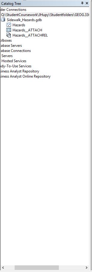
Once the fields and domains were created, the attachment option was employed (figure 4). This new feature class was brought into ArcMap and subsequently published to ArcGIS Online so it could be utilized by Arc Collector.

Figure 4. Catalog tree showing the picture attachment option added to the geodatabase.

The map is now ready to be used by Arc Collector. Using an iPhone, data points were collected on the sidewalks in Randall Park and uploaded to the feature class in the online map. Several photos were also taken to aid in hazard determination (figure 5).

Figure 5. a) Map with data points on the Arc Collector app. b) Data point fields in the Arc Collector app.

After data collection the data was analyzed in ArcMap for hazard determination.

Results/Discussion

Above is the online map created to house the hazard data. Each data point can be clicked and the attribute information as well as any attachments can be viewed. From the map, one can see some areas have a higher density of sidewalk hazards than others. However, this trend and others are more clearly seen in the following figures.

Figure 6. Map of sidewalk hazards in Randall Park in Eau Claire, WI.

Figure 6 shows the different types of hazards recorded in Randall Park. This map shows that there are indeed sidewalk hazards in Randall Park and it shows where certain types of hazards are located. Besides just hazard identification, some trends in hazard locations can also be derived. The eastern side of the park has markedly less hazards than the southern or eastern side of the park. This sidewalk was clear of snow or ice and had no noticeable bumps or other hazards. The southern end of the park had a high concentration of snow or ice on the sidewalk. This appeared to be due to insufficient plowing. The outside sidewalk also showed more hazards than the two arching sidewalks within the park. This makes sense because students walking in the area are more likely to walk around the outside to get to their destination rather than through the park.

Figure 7. Map of snow or ice sidewalk coverage in Randall Park, Eau Claire, WI

Figure 7 shows the percentage of snow or ice coverage on the sidewalk. The largest coverage was inside the part around the center square. One portion of the walkway was not plowed at all. There was a higher concentration of snow on the southeast corner, but the other concentrations of snow were minimal. Most of the snow or ice piles were due to shade from trees or a crooked plowing course, both of which were recorded in the field.

Conclusions

This lab emphasizes the need for proper planning before a project is initiated. During data collection, it is almost impossible to go back and re-configure the geodatabase to suit the needs of the project, especially in the field. If the project is not well-defined, then the data collected will be insufficient to answer the question and complete the objectives. In this exercise it was determined that there were sidewalk hazards in Randall Park of Eau Claire, WI. The types of hazards and extent of the hazards were also determined. This small study indicates that the sidewalks in Eau Claire, particularly in high student traffic areas, are in need of repairs. The database provides sufficient data for the city to make the necessary repairs to provide better amenities for a large percentage of the Eau Claire population.

With more time, a larger sample size that includes more of the student neighborhoods would be included in the analysis. This would further clarify the condition of sidewalks in student living areas. If the project were repeated, a new option that allows the data collector to select more than one damage type per data point would be added because some of the hazards were paired together such as a rough surface and uneven slope. The ability to denote more than one hazard type would also aid in expediting the data collection process. Data collection could also be expanded to UW-Eau Claire students so they could identify sidewalk hazards on their daily commute. This would extend the scale of hazard analysis. Overall, this project has shown that Arc Collector is a great tool for field studies and has applications in city maintenance projects, particularly sidewalk maintenance.