Lab 3: Creation of Navigation Maps

Introduction

Navigation has come far since the first naval maps were created with the advent of geospatial technologies. However there is still merit in learning how to use physical navigation maps. The purpose of this lab was to create two navigation maps to be used in a future exercise.  These maps must reference a location system which consists of a coordinate system and a projection. A geographic coordinate system is a three-dimensional reference system that assists in locating points on the Earth’s surface. Coordinate systems are also important in framing the area where desired objects are located.  A map projection is the transformation of the earth, a three-dimensional object, to a flat surface. The projection's purpose is to display the data. In this activity one map uses the WGS_1984_Web_Mercator_Auxiliary_Sphere coordinate system in the Mercator_Auxiliary_Sphere projection and the other map uses the WGS_1984_UTM_Zone_15N coordinate system in the Transverse Mercator projection.

Study Area

The study area is a section of land owned by the University of Wisconsin–Eau Claire called the Priory (figure 1). This area is just south of Highway 94 and east of West Lowes Creek Rd in Eau Claire, WI.  The Priory includes 120 acres of wooded area as part of the children’s nature academy which constitutes a large amount of the mapped area. The navigation boundary included in the Priory_Database is approximately 862,500 square meters.

Figure 1. Navigation map study area surrounding the Priory in Eau Claire, WI.

Methods

The first step in this lab was to identify the two coordinate systems for the maps. The coordinate system provides the framework for defining the real-world locations that will later be identified. A number of factors define a coordinate system. The first factor is its measurement framework.  There are two main categories: geographic or planimetric. A geographic system has spherical coordinates that are measured from earth’s center and a planimetric system projects the coordinates onto a two-dimensional surface. The following factors are units of measurement, type of map projection, and the other miscellaneous properties such as datums, standard parallels, central meridians, and shifts in the x and y directions.

Universal Transverse Mercator (UTM) Coordinate System

The first map utilized a UTM coordinate system. UTM uses a cylinder and divides the ellipsoid into 60 different wedges.  Each of these wedges includes 6° of longitude and has its own central meridian. The UTM zone closest to the area of study must be selected to minimize distortion. In this case, UTM Zone 15N is used (figure 2). This coordinate system is based on the WGS 1984 geographic coordinate system. 

Figure 2. Example of UTM zones in the contiguous United States.

Web Mercator Auxiliary Sphere Coordinate System

The second map created utilized WGS_1984_Web_Mercator_Auxiliary_Sphere. The Web Mercator is the standard for any online map to maintain consistency across platforms. This coordinate system uses spherical formulas at all scales whereas large-scale Mercator maps normally use the ellipsoidal form of the projection.  Each point on the map has two coordinate values: latitude and longitude that indicate the angle from the center of the earth. Figure 3 demonstrates this concept. This coordinate system was used because it creates straight grid lines.

Figure 3. Example of how latitude and longitude values are derived from a geographic coordinate system.

 Map Creation

The actual creation of the maps involved the creation of contour lines and a grid to provide a frame of reference when the map is used for navigation. All the data for the maps was provided by Dr. Hupy in the priory geodatabase (figure 4).

Figure 4. Priory geodatabase with all the data needed for this lab.

First the priorylidar raster was added to the main window. This raster was previously mosaicked from three separate rasters to enable easier processing. A polygon feature class of the navigation boundary was also added for context. Both are shown in figure 5. Based on the priorylidar, the contour tool was used to create 10 foot contours. This tool creates a line feature class of contours (isolines) from a raster surface. The contours were in feet because the priorylidar raster is projected in NAD_1983_HARN_WISCRS_EauClaire_County_Feet.

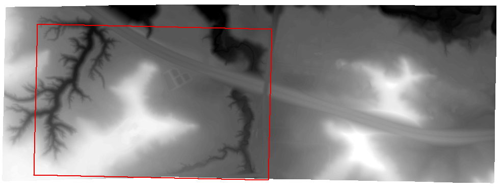Figure 5. Priorylidar and navigation boundary before processing.

 Before further processing, the navigation boundary was projected using the project tool and the priorylidar raster was projected using the project raster tool. The project tool projects spatial data from one coordinate system to another. The project raster tool transforms a raster into a new projection and creates a new raster. This was done twice for each coordinate system used. and ensures that there are no discrepancies between the data layers and the navigation data collected later is spatially accurate.
 
 Caution was taken to not use project define, which overwrites the coordinate system information stored in a data set. This causes problems if the coordinate system named is not the coordinate system of the data. This error is analogous to calling someone “Beth” when their name is actually “Lisa.”

Next, a grid was created using data frame properties. For the UTM map, a measured grid based on UTM was included that has grid lines spaced 50 meters apart. The decimal degrees map had a graticule grid based on latitude/longitude with decimal degrees as the label out to four decimal places. To do this, within data frame properties the grid tab was selected and the correct measurements were confirmed for each map (figure 6). 

Figure 6. Grid properties for the measured grid used in the UTM map.

The final step was adding cartographic elements to each map including the following:

• North arrow
• Scale bar
• Representative Fraction Bar
• Description of projection and coordinate system
• List of data sources
• Watermark
• Contour

 The map was then formatted to 11x17 in size and landscape format.

Results

 The result was two navigation maps with different coordinate systems and grids to aid in a navigation activity at a later date (figure 7 and figure 8).

Figure 7. UTM Priory Navigation Map.

Figure 8. Decimal Degrees Priory Navigation Map.

Depending on the coordinate system used, the grid lines changed due to differences in measurements. Both maps were kept blank except for the contour and grid lines to ensure easy reading when used in the field.

Conclusion

This lab provided the knowledge of how to create a navigation map using different types of coordinate systems. Despite advances in technology, there are still times when physical maps are necessary. The lab also provided the opportunity to discern which cartographic symbols are necessary for a field map. Overall it is important to understand the other methods of navigation that exist outside of technology sources such as GPS.

Sources

 Define Projection. (n.d.). Retrieved February 14, 2018 fromhttp://pro.arcgis.com/en/pro-app/tool-reference/data-management/define-projection.htm
 Project. (n.d.). Retrieved February 14, 2018 from http://pro.arcgis.com/en/pro-app/tool-reference/data-management/project.htm
Project Raster. (n.d.). Retrieved February 14, 2018 from http://pro.arcgis.com/en/pro-app/tool-reference/data-management/project-raster.htm
Contour. (n.d.). Retrieved February 14, 2018 from http://pro.arcgis.com/en/pro-app/tool-reference/spatial-analyst/contour.htm
Coordinate systems, map projections, and geographic (datum) transformations. (n.d.). Retrieved February 14, 2018 from http://resources.esri.com/help/9.3/arcgisengine/dotnet/89b720a5-7339-44b0-8b58-0f5bf2843393.htm
What is a Coordinate System? (n.d.). Retrieved February 14, 2018 from http://edndoc.esri.com/arcsde/9.1/general_topics/what_coord_sys.htm