Lab 10: Distance Azimuth Survey

Introduction

Sometimes technology can fail in the field and another method is needed to complete the work. This lab introduced the distance azimuth survey, a basic survey technique that can come in handy if such a circumstance arises. This sampling technique is related to others such as the point-quarter method or mapping out linear features on the landscape. In this lab groups of three to four students went out to Putnam drive on the University of Wisconsin-Eau Claire campus and completed a tree survey to practice the distance azimuth survey technique. The data was then inputted to ArcMap and transformed into a feature class that could be further analyzed.

Study Area

The study area was located on Putnam Drive behind the University of Wisconsin-Eau Claire (figure 1).

Figure 1. Putnam Drive in Eau Claire, WI where the tree survey was completed.

This area is populated with both dry and wet soil trees. The area directly adjacent to the parking lot behind Davies Center on campus is a small swamp with a small stream flowing along its border. Across the swamp is a gravel trail accessible to cars and bikers. Beyond this trail is the steep incline that leads to the former flood plain of the Chippewa River called the Wissota Terrace, or better known as upper campus. The swamp area has wet soil species such as river birch and ash trees. The steep incline leading to upper campus has a drier soil due to water running to lower elevation areas. This section of Putnam trail is home to dry soil species such as red oak and basswood trees. The trees selected for this tree survey were located in both areas. Trees selected for the survey were chosen based on distance from the reference point (had to be feasible to measure the distance from reference point) and the tree type (several tree types were desired for the survey).

Methods

The attributes collected for each point were chosen before sampling to ensure usable data was collected. In this survey, 17 trees were sampled. The location column in the data was recorded for the reference point and thus was the same for the first 12 trees and again for the remaining 5 due to the nature of the distance azimuth survey. In addition, the distance from the reference point, azimuth (degree angle from north), tree type, and circumference were all recorded for each tree. The azimuth and distance will be described shortly in the survey process. Tree type and circumference were chosen as tree characteristics that could later be analyzed spatially for any patterns on the maps in relation to topography and soil type

The process for collecting each tree sample was as follows. First, a reference point was established. The coordinates for this point were obtained using Bad Elf GPS and an iPhone. Bad Elf was used to collect the second reference point as well (figure 2).

Figure 2. Bad Elf GPS device used with an iPhone to obtain reference point coordinates.

Next, a tree was chosen based on location and tree type. The tree was identified based on its bark and leaves. Once the tree was chosen, a tape measure determined the circumference of the tree in centimeters. Then, the tape measure was used to determine the tree’s distance from the reference point (figure 3).

Figure 3. Tape measure used to determine the distance of each tree from the reference point. The reference point is located where the two individuals are standing in the background.

For some tree distances, a laser was used but it was found to be more inaccurate than the tape measure so its use was discontinued. Finally, the azimuth was determined using a field compass (figure 4).

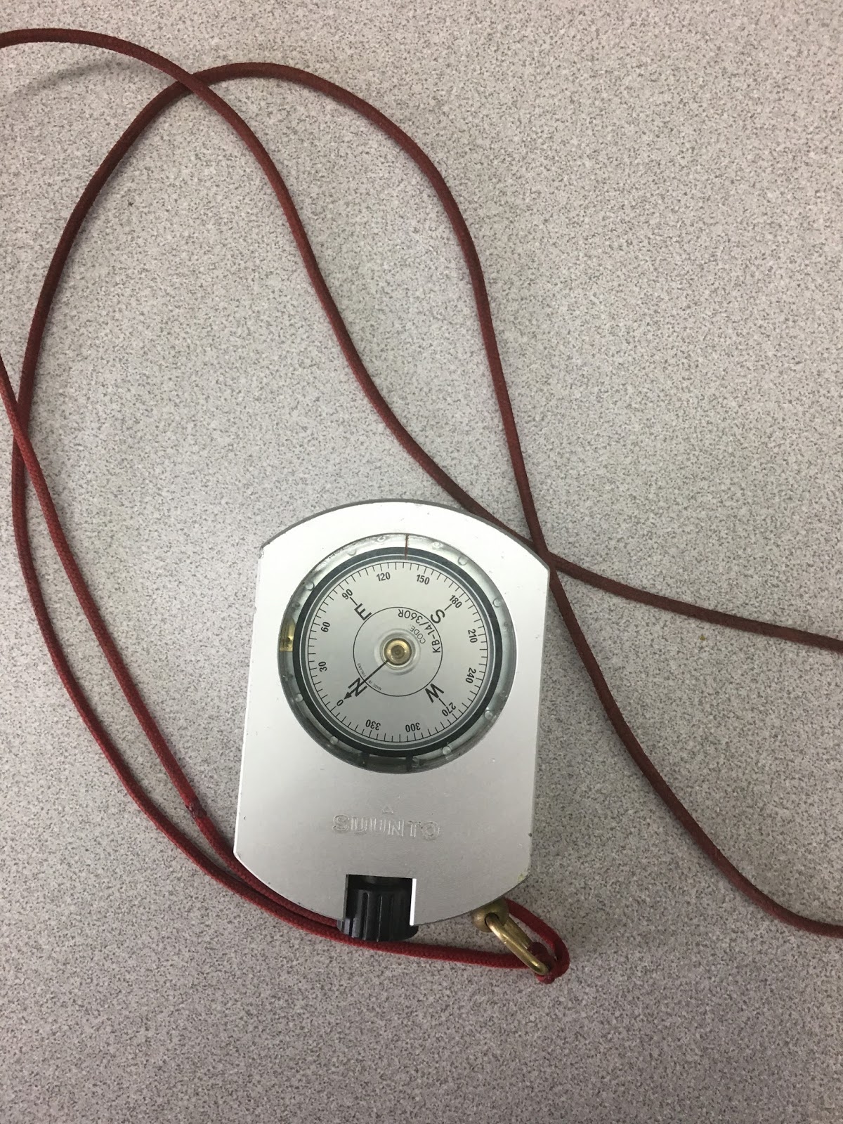Figure 4. Azimuth compass used to determine the azimuth of each tree sample.

By looking through the azimuth compass, the degree measure from north, or 0 °, can be accurately obtained as demonstrated in figure 5.

Figure 5. Azimuth compass used by Luke Burds to obtain an azimuth reading.

Figure 6 shows the complete table of all measurements taken in the field. The left page describes what each symbol represents for the tree types in the table on the right-hand page.

Figure 6. Field notebook including all data obtained for each tree sample.

With this information and the distance from the reference point, the x, y coordinates can be obtained in ArcMap. 

The final step was to import the data into an excel file and then to ArcMap and run two tools: Bearing Distance to Line tool and Feature Vertices to Points tool. Both of these tools are located in the ‘data management tool box’ and under the ‘feature’ subset. The bearing distance to line command creates a new feature class containing geodetic line features constructed based on x, y, azimuth, and distance values. In other words, lines from the reference point are plotted based on the x, y coordinates of the reference point and the azimuth and distance of each tree surveyed. This tool also allows the user to import other attribute data field information such as the tree type.

Next, the Feature Vertices to Points tool created a feature class containing points generated from the specified locations at the ends of the lines that were created with the previous tool. This then creates a point feature class that contains all the pertinent attribute data that can be used for querying in the future. 

Results/Discussion

Figure 7. Map of lines from the reference point to each tree location. There were two separate data groups.

Figure 7 shows the line feature class that was created using the bearing distance to line tool. Each line originates from the reference point and ends at the tree location. This feature class lines up with survey data taken.

Figure 8. Map of tree locations in Putnam Drive. These locations were derived from the locations denoted at the ends of the lines in the map in figure 7.

Figure 8 shows the final points depicting tree locations. The points are fairly accurate based on the basemap imagery. Some of the tree sampled down in the swamp area appear to be on the path, but this discrepancy could be due to the change in elevation not included in the basemap.  In particular, the points are very accurate location-wise from the reference point. This accuracy and overall accuracy in the real-world indicate that the measurements were accurate as were the GPS coordinates.

Figure 9. Tree types denoted by color. No apparent trends are seen in the data.

Figure 9 shows the tree types of the 17 trees sampled in the survey. The sample size is quite small, so no trends such as wet vs. dry soil tree types appear in the data.  However, there was one river birch in the right-hand sample and two black walnut in the left-hand sample. Both these trees did occur at a lower frequency than the other types of trees based on a visual analysis of the area.

Conclusion

Overall this lab was effective in providing experience in performing a distance azimuth survey. This technique is beneficial because it can be used in the field when other forms of technology are unavailable and can also be very accurate as the results showed. A survey would take more time if the objects were a farther distance away than 20 meters. This used to be the standard technique used in the field to collect data. Today, survey-grade GPS units have replaced this method with accurate locations down to the centimeter in certain cases. GPS units today can also do post-processing in addition to gathering the initial data. While easier methods for obtaining field data are available, the distance-azimuth method is still a valuable tool in obtaining data if technology fails (which it can and will) in the field.

Sources

“Bearing Distance to Line.” (2018). Accessed April 24, 2018. http://pro.arcgis.com/en/pro-app/tool-reference/data-management/bearing-distance-to-line.htm

“Feature Vertices to Points.” (2018). Accessed April 24, 2018. http://pro.arcgis.com/en/pro-app/tool-reference/data-management/feature-vertices-to-points.htm