Lab 2: Visualizing a Terrain Survey

Introduction

In the previous lab the group designed and created a terrain in a sandbox to practice surveying techniques. The group went outside, created the terrain in a sandbox, and proceeded to make a 20 by 20 box grid out of string for systematic sampling (there were only 18 points sampled each way). To read more about the methods and results please see lab one.

Lab two is a continuation of lab one in which the data previously collected was imported to ArcMap and ArcScene to visualize the data points. The goal was to determine if the sampling method was sufficient to capture the created terrain and to determine which visualization method best matches the survey data.  Before this could be completed, the data had to be normalized.  Data normalization is organizing data and correcting data entry errors to further analyze it (Database Normalization Explained in Simple English).  Data normalization for the group consisted of creating three columns (x, y, z) out of the data so it could be imported into ArcMap (Figure 1).

Figure 1. Survey data separated into three columns (x, y, z) during data normalization. This allowed the data to be imported into ArcMap. Note the z values corrected to positive numbers from negatives.

It is important to know not only how to survey an area but also how to portray the data afterwards. Interpolation is one way to visualize data.  Different methods will connect the values in a different manner to create a continuous surface. The interpolation methods used in this lab will render a surface based on the location and magnitude of z values.  The various interpolation methods helped the group determine how well the terrain was surveyed and where two columns were missed in the survey.

Methods

The first step in visualizing the data was data normalization mentioned above.  In addition, all values in the columns were converted to numeric in excel and the number of decimals was set to one.  Then in ArcMap a file geodatabase was created to hold all the feature classes and raster files created throughout the lab.  Once the geodatabase was created, the table of the data was imported from excel.  The 'add XY data' function was used to display the data as an event.  Figure 2 shows how the survey points looked after this function was completed.

Figure 2. Survey points as an XY event in ArcMap. The two missing columns are apparent because the grid should have been 18 by 18. 

The data (Figure 2) shows up in a systematic sampling pattern, so it was then converted to a feature class for further analysis. During the conversion a coordinate system was not specified.  A coordinate system was not specified because this data has a cadastral coordinate system, otherwise known as its own coordinate system. The origin from which all (x, y) points were measured was relative to the sandbox, not a global coordinate system, so projecting the data would not place the data points correctly on the earth's surface. 

After the feature class was created, five different interpolation methods were executed on the data: IDW, Natural Neighbors, Kriging, Spline, and TIN. All these methods resulted in the creation of a new raster representing the terrain surface created in the sandbox.

• IDW (Inverse distance weighted)
• this method determines cell values based on the points surrounding it 
• Nearer points have more influence on the cell value than farther points
• the advantage of IDW is that by defining a power value, one can control whether nearer points have more influence (more detail but less smooth) or if farther points have more influence (less detail but smoother)
• the disadvantage of IDW is that the formula used isn't connected to any natural phenomena, so there isn't a way to determine whether a power value is too big or too small
•  Natural Neighbors
• in this method surface points are a result of nearby points or "neighbors"
• creates polygons out of the given points, creates a polygon around the interpolation point, and assigns weights to the given points based on how much the polygons overlap
• the advantage of natural neighbors is that point values are assigned based on local values only and will create a smooth surface 
• the disadvantage of natural neighbors is it does not infer trends and won't produce changes in the surface if they weren't already recorded in the data
•  Kriging
• perhaps the most complicated, kriging is a geostatistical method that includes statistical relationships among the points and thus creates a predictive surface map
• a mathematical function is fit to a specified number of points or all points withing a specified radius to determine the output value for each location (similar to IDW but more sophisticated)
• kriging is a good model if more accurate interpolation is needed such as including  trends in data
• kriging's disadvantage is its complexity which limits its use to only those who thoroughly understand its mechanics
•  Spline 
• spline estimates the surface using a mathematical equation that both minimizes curvature and passes exactly through all data points
• the advantage of spline is its ability to create a smooth surface based on every point
• because of its smoothing function spline does not represent small changes in elevation well
•  TIN
•  this method is a form of vector-based digital geographic data 
• creates triangles out of vertices (data points) 
• TINs are adept at showing a highly variable surface like a ridge or mountain
• The disadvantage is a high volume of data that can quickly become too large to save in a geodatabase 

 After each interpolation was executed, a hillshade raster was created to underlay the interpolation raster for more definition.  These were all placed on one map document with north facing up and a scale bar, north arrow, and legend. Scale for each image is shown as a drawn scale bar along the bottom that represents the distance in centimeters of the actual sandbox surveyed. both orientation and scale are needed in these images because without the addition of a north arrow or scale, the image cannot be considered a map. Then each interpolation raster was imported to ArcScene for 3D viewing.  The elevations in ArcScene for each raster were set to float on a custom surface and visibility was set to render the layer at all times. If possible, areal features were smoothly shaded relative to the scene's light position.  Once a 3D image was completed, it was exported as a PNG file.

Results and Discussion

For reference, Figure 3 shows the original terrain created in the sandbox.  This will be used to decide how well each interpolation method recreated the terrain surface.

Figure 3. Completed terrain surface in sandbox.

Figure 4 is the final map comparing all five interpolation methods against each other.  These will be discussed separately and compared to the original terrain model.

Figure 4. Map of all five interpolation methods. A legend of the spline interpolation method is included as a general example for all five methods.

Figure 5. Image of the spline interpolation method in ArcScene.

The spline interpolation method (Figure 5) did a good job showing overall elevation changes in the terrain. the smoothness of this model gives the best view of the smiley face the group was trying to create.  The spline method does remove some more pronounced elevation changes, but the original design had more attenuated slopes to begin with so this was an accurate reflection of the surface.  In addition, the spline method is by far the most aesthetically pleasing of all the methods.

Figure 6. Image of the IDW interpolation method in ArcScene.

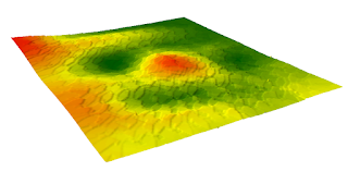
The IDW interpolation method (Figure 6) did not give as aesthetically pleasing of an image as the spline method.  The surface appears bubbly which gives the impression there were multiple peaks (this was not the case).  This method excels at correctly showing the elevation of the data points but does a poor job in representing the elevations between points.  Overall this method does not represent the surface well. 

Figure 7. Image of the Natural Neighbors interpolation method in ArcScene.

The natural neighbors interpolation method (Figure 7) looks like a cross between the spline and IDW methods.  The terrain features that the group created were very smooth, so this method was able to capture the ridge, hill, valley and depression quite well. Smaller changes in elevation are not as accurately portrayed in this method because interpolation points are only dependent on points within a certain distance of it.  Overall this method does well showing the terrain but does not provide as good of definition of features as the spline method. 

Figure 8. Image of the Kriging interpolation method in ArcScene.

The kriging method (Figure 8) was by far the least accurate of all the methods.  The geometric approach of this method meant that more prediction and statistical figures were used in determining elevations.  The depressions and hills are hard to see and it looks like circles are placed over each other across the surface.  The smiley face is least noticeable with the kriging method.

Figure 9. Image of the TIN interpolation method in ArcScene.

The TIN method (Figure 9) did a good job of geometrically representing the surface.  This method does the best job of showing multiple faces of terrain features such as the hill in the center. However, all the features appear sharper than they were in the sandbox because the surface is created out of triangles. For this terrain made of curving features, the TIN model does not accurately depict it.  

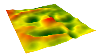
Out of all the methods discussed above, the spline interpolation method did the best job of representing the terrain surface originally built.  The smoothness of the features was a good representation of the attenuated curves of the sand structures that lacked definition.  In addition, all the methods showed the survey error to a degree, but the spline method showed the area of error the best.  In figure 5, the right-hand side of the smiley face looks distorted.  The right eye does not show up, the eyebrow disappears, and the right side of the mouth is not defined.  This was most likely where two columns of data were missed.

 Conclusion

In the previous lab a terrain was created and elevation points were systematically recorded.  The data points were then normalized and placed into ArcMap.  The subsequent table was converted to a feature class and subjected to five interpolation methods. This was completed because these data points have no meaning unless they are placed into a program such as ArcMap or ArcScene where the different elevations can be visualized.

Other field based surveys will use the same general workflow as lab 1 and lab 2 to create 3D surfaces of a terrain on the earth's surface.  There are also similar issues such as data consistency and propagation of errors in models that were present in the initial data.  There are minor differences such as the method of dividing the terrain. The string and thumbtacks used in this lab would not be reasonable for modeling real world terrain.  In addition, detailed grid surveys are not always possible because of constraints on time, money, and resources.  The interpolation methods mentioned in this lab have applications beyond just elevation, such as precipitation and temperature values.  An example of interpolation methods being used for rainfall can be viewed in one of my previous projects here. Overall this lab helped introduce surveying techniques and methods for visualizing survey data points via interpolation.

Sources

Database Normalization Explained in Simple English. (n.d.). Retrieved February 7, 2018, from https://www.essentialsql.com/get-ready-to-learn-sql-database-normalization-explained-in-simple-english/
How IDW Works. (n.d.). Retrieved February 7, 2018 from http://desktop.arcgis.com/en/arcmap/10.3/tools/3d-analyst-toolbox/how-idw-works.htm
How Natural Neighbors Works. (n.d.). Retrieved February 7, 2018 from http://desktop.arcgis.com/en/arcmap/10.3/tools/3d-analyst-toolbox/how-natural-neighbor-works.htm
How Kriging Works. (n.d.). Retrieved February 7, 2018 from http://desktop.arcgis.com/en/arcmap/10.3/tools/3d-analyst-toolbox/how-kriging-works.htm
How Spline Works. (n.d.). Retrieved February 7, 2018 from  http://desktop.arcgis.com/en/arcmap/10.3/tools/3d-analyst-toolbox/how-spline-works.htm
What is a TIN Surface? (n.d.) Retrieved February 7, 2018 from  http://desktop.arcgis.com/en/arcmap/10.3/manage-data/tin/fundamentals-of-tin-surfaces.htm